Reinforcement Learning

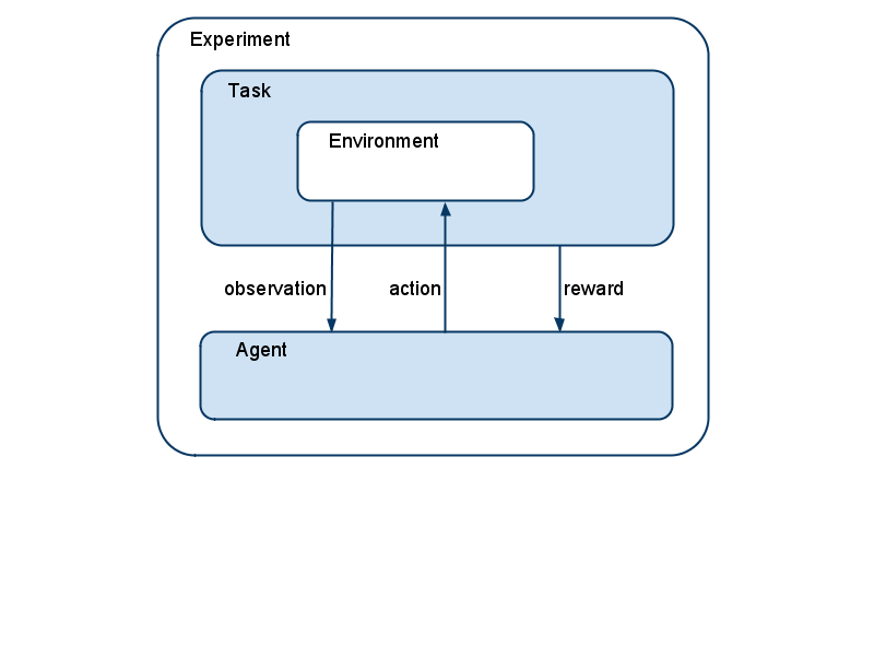
A reinforcement learning (RL) task in PyBrain always consists of a few components that interact with each other: Environment, Agent, Task, and Experiment. In this tutorial we will go through each of them, create the instances and explain what they do.

But first of all, we need to import some general packages and the RL components from PyBrain:

from scipy import *
import sys, time

from pybrain.rl.environments.mazes import Maze, MDPMazeTask
from pybrain.rl.learners.valuebased import ActionValueTable
from pybrain.rl.agents import LearningAgent
from pybrain.rl.learners import Q, SARSA
from pybrain.rl.experiments import Experiment
from pybrain.rl.environments import Task

Note

You can directly run the code in this tutorial by running the script docs/tutorials/rl.py.

For later visualization purposes, we also need to initialize the plotting engine (interactive mode).

import pylab
pylab.gray()
pylab.ion()

The Environment is the world, in which the agent acts. It receives input with the performAction() method and returns an output with getSensors(). All environments in PyBrain are located under pybrain/rl/environments.

One of these environments is the maze environment, which we will use for this tutorial. It creates a labyrinth with free fields, walls, and an goal point. An agent can move over the free fields and needs to find the goal point. Let’s define the maze structure, a simple 2D numpy array, where 1 is a wall and 0 is a free field:

structure = array([[1, 1, 1, 1, 1, 1, 1, 1, 1],
                   [1, 0, 0, 1, 0, 0, 0, 0, 1],
                   [1, 0, 0, 1, 0, 0, 1, 0, 1],
                   [1, 0, 0, 1, 0, 0, 1, 0, 1],
                   [1, 0, 0, 1, 0, 1, 1, 0, 1],
                   [1, 0, 0, 0, 0, 0, 1, 0, 1],
                   [1, 1, 1, 1, 1, 1, 1, 0, 1],
                   [1, 0, 0, 0, 0, 0, 0, 0, 1],
                   [1, 1, 1, 1, 1, 1, 1, 1, 1]])

Then we create the environment with the structure as first parameter and the goal field tuple as second parameter:

environment = Maze(structure, (7, 7))

Next, we need an agent. The agent is where the learning happens. It can interact with the environment with its getAction() and integrateObservation() methods.

The agent itself consists of a controller, which maps states to actions, a learner, which updates the controller parameters according to the interaction it had with the world, and an explorer, which adds some explorative behavior to the actions. All standard agents already have a default explorer, so we don’t need to take care of that in this tutorial.

The controller in PyBrain is a module, that takes states as inputs and transforms them into actions. For value-based methods, like the Q-Learning algorithm we will use here, we need a module that implements the ActionValueInterface. There are currently two modules in PyBrain that do this: The ActionValueTable for discrete actions and the ActionValueNetwork for continuous actions. Our maze uses discrete actions, so we need a table:

controller = ActionValueTable(81, 4)
controller.initialize(1.)

The table needs the number of states and actions as parameters. The standard maze environment comes with the following 4 actions: north, south, east, west.

Then, we initialize the table with 1 everywhere. This is not always necessary but will help converge faster, because unvisited state-action pairs have a promising positive value and will be preferred over visited ones that didn’t lead to the goal.

Each agent also has a learner component. Several classes of RL learners are currently implemented in PyBrain: black box optimizers, direct search methods, and value-based learners. The classical Reinforcement Learning mostly consists of value-based learning, in which of the most well-known algorithms is the Q-Learning algorithm. Let’s now create the agent and give it the controller and learner as parameters.

learner = Q()
agent = LearningAgent(controller, learner)

So far, there is no connection between the agent and the environment. In fact, in PyBrain, there is a special component that connects environment and agent: the task. A task also specifies what the goal is in an environment and how the agent is rewarded for its actions. For episodic experiments, the Task also decides when an episode is over. Environments usually bring along their own tasks. The Maze environment for example has a MDPMazeTask, that we will use. MDP stands for “markov decision process” and means here, that the agent knows its exact location in the maze. The task receives the environment as parameter.

task = MDPMazeTask(environment)

Finally, in order to learn something, we create an experiment, tell it both task and agent (it knows the environment through the task) and let it run for some number of steps or infinitely, like here:

experiment = Experiment(task, agent)

while True:
    experiment.doInteractions(100)
    agent.learn()
    agent.reset()

    pylab.pcolor(controller.params.reshape(81,4).max(1).reshape(9,9))
    pylab.draw()

Above, the experiment executes 100 interactions between agent and environment, or, to be exact, between the agent and the task. The task will process the agent’s actions, possibly scale it and hand it over to the environment. The environment responds, returns the new state back to the task which decides what information should be given to the agent. The task also gives a reward value for each step to the agent.

After 100 steps, we call the agent’s learn() method and then reset it. This will make the agent forget the previously executed steps but of course it won’t undo the changes it learned.

Then the loop is repeated, until a desired behavior is learned.

In order to observe the learning progress, we visualize the controller with the last two code lines in the loop. The ActionValueTable consists of a scalar value for each state/action pair, in this case 81x4 values. A nice way to visualize learning is to only consider the maximum value over all actions for each state. This value is called the state-value V and is defined as V(s) = max_a Q(s, a).

We plot the new table after learning and resetting the agent, inside the while loop. Running this code, you should see the shape of the maze and a change of colors for the free fields. During learning, colors may jump and change back and forth, but eventually the learning should converge to the true state values, having higher scores (brighter fields) the closer they are to the goal.